During the summer of 2021, Chumeng Di, Ethan Levin, and Arie Ogranovich, took part in an undergraduate research project funded by the NSF grant DMS 2005501 aimed at visualizing planar maximal surfaces in anti-de Sitter space.
In a recent paper, I proved that there is a homeomorphism between the moduli space of polynomial holomorphic quadratic differentials of degree k on the complex plane and light-like polygons with 2k+4 vertices in the Einstein Universe. The proof is based on the fact that given a polynomial holomorphic quadratic differential \( q \), there is a unique maximal surface in anti-de Sitter space that is conformally planar and whose second fundamental form is the real part of \( q \). In theory, the construction is quite explicit:
- we find a function \( u:\mathbb{C} \rightarrow \mathbb{R} \) such that the pair \( (2e^{2u}|dz|^2, 2\mathcal{Re}(q)) \) satisfies the Gauss-Codazzi equations for surfaces in anti-de Sitter space. This amounts to solving the PDE: \( \Delta u = 2e^{2u}-2e^{-2u}|q|^{2} \).
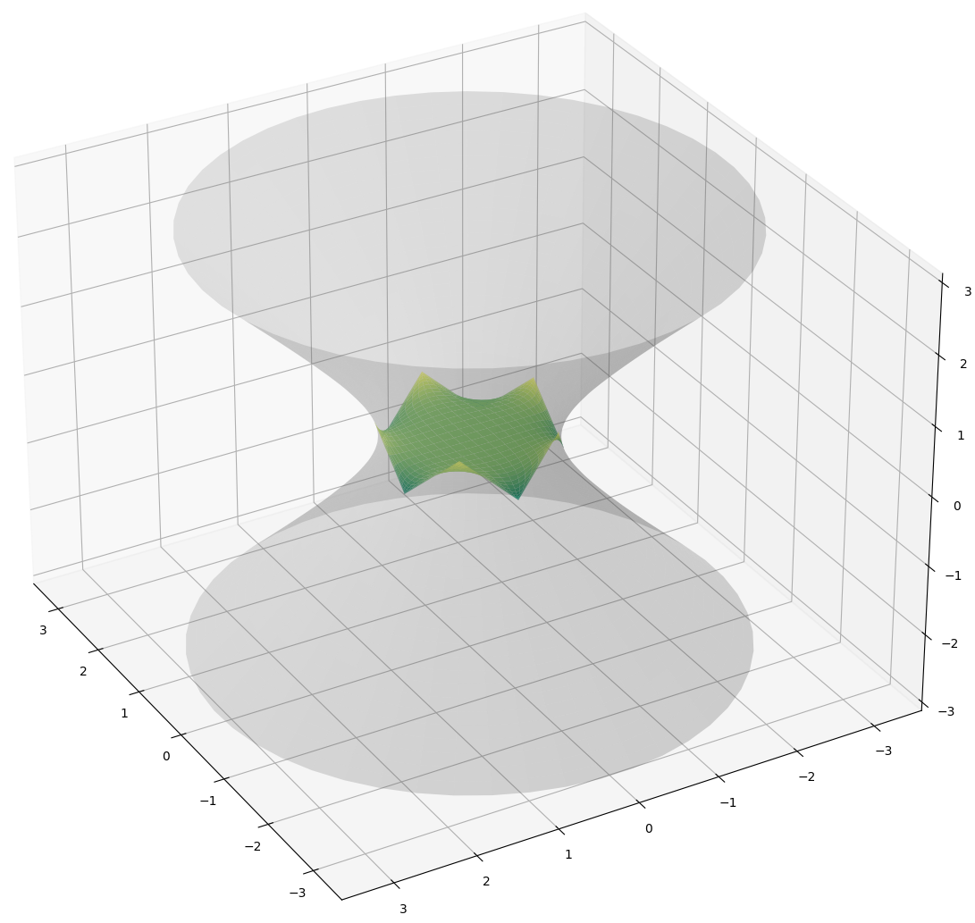
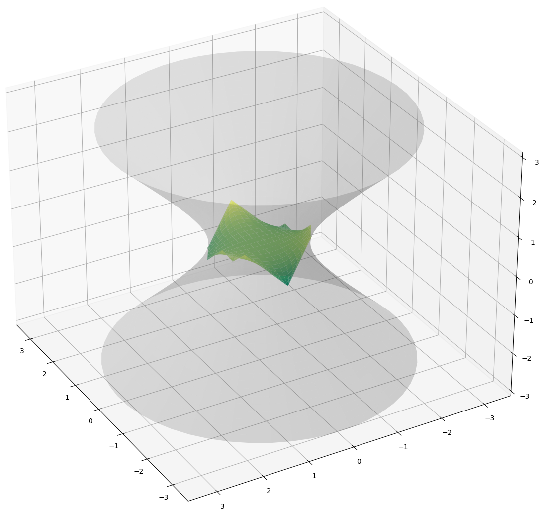
- the fundamental theorem of surfaces furnishes then a maximal embedding \( f: \mathbb{C} \rightarrow \mathrm{AdS}^{3} \) with induced metric \( 2e^{2u}|dz|^{2} \) and second fundamental form \( \mathrm{II}=2\mathcal{Re}(q). \) The frame field of \( f \), i.e. the matrix \( F\) with columns \( f, f_{x}, f_{y}, N\), where \( N\) is the unit normal vector to the surface, satisfies an ODE of the form \( F^{-1}dF= Udx+Vdy \), with \(U\) and \(V\) explicit and written in terms only of \( u\) and \(q\).
- Solving the above ODE gives then a matrix \( F\) whose first column is a parameterization of the maximal surface associated to the polynomial holomorphic quadratic differential \( q\). The boundary of this surface is a light-like polygon in the Einstein Universe.
 |
 |
In the second part of the project, we studied how the light-like polygons on the boundary vary when we change the coefficients of the polynomial. We focused on two cases in particular: when we rotate the polynomial, i.e we consider the family \( e^{i\theta} q\) for a fixed holomorphic quadratic differental \(q \); and when we rescale the polynomial by \( t \in \mathbb{R} \) and we tend \( t \) to \( +\infty \). We produced some animations for these families of polygons. Here below you may find two examples, corresponding to \( e^{i\theta}(z^2+1)dz^2 \) (on the left) and \( t(z^3+z)dz^2 \) (on the right):
For a more detailed account of the project, please refer to the final report or the poster presentation summarizing this work.